Before the Order: Which Books Belong Nearby?

My order begins before I click Buy. Someone has already decided whether Maya's book deserves space near me. Too few copies can mean an expensive rescue shipment or a lost sale. Too many can leave Maya financing books that do not move.

Three decisions sit behind the shelf. Forecasting describes possible demand. Assortment selects the titles to carry locally. Placement chooses quantities and locations. A better prediction is useful only if it improves those choices.

Sales are what happened under the old offer

If Maya's book was unavailable for a week, zero recorded sales do not prove zero demand. If a faster promise changes conversion, demand under the new promise may differ from historical sales. Price, promotions, availability, and service affect the observations used to learn demand.

A useful forecast therefore states the horizon, geography, product, and conditions it represents. Leaders need to know whether they are looking at demand under the present policy or an estimate of demand under a proposed one. More sophisticated machine learning does not remove this distinction.

Why an average can choose the wrong stock level

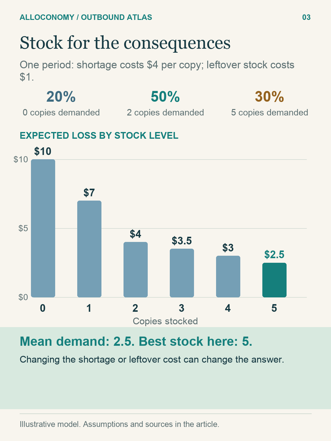
Take a separate, invented one-period example. Demand for a title is zero with probability 20%, two with probability 50%, and five with probability 30%. Average demand is 2.5 copies, but copies are not divisible and shortages and leftovers have different consequences.

Assume each unmet unit causes $4 of incremental loss and each leftover causes $1. These are stipulated economic penalties relative to a common baseline, including the relevant purchase and recovery effects; they are not the book's selling price.

Stock	Expected shortage loss	Expected leftover loss	Total expected loss
2 copies	30% × 3 × $4 = $3.60	20% × 2 × $1 = $0.40	$4.00
5 copies	$0	20% × 5 × $1 + 50% × 3 × $1 = $2.50	$2.50

In this simple model, choose the smallest quantity whose cumulative demand probability reaches shortage penalty ÷ (shortage penalty + leftover penalty): 4 ÷ 5 = 80%. Demand of two covers only 70% of outcomes, so five wins. Checking all quantities from zero to five confirms it. This is a one-period teaching rule, not a universal service target. Storage limits, replenishment, substitution, and multiple periods change the problem.

The first local copy is different from the hundredth

Assortment asks whether a title deserves local presence at all. The first nearby copy might avoid a remote shipment and enable a faster offer. Later copies protect increasingly unlikely demand. A bulky machine can consume space needed for many books, even when its sales value is higher.

Rankings should reflect the constrained resource. If shelf space is scarce, compare incremental benefit per relevant space requirement. If receiving or packing is scarce, space alone is the wrong denominator. Complements complicate the calculation: a printer and compatible consumables can create value together that separate rankings miss.

One way to coordinate many products is a scarcity price for shared space. Each product's model responds to that price; the coordinator raises it when total requested space exceeds capacity. This is a mathematical coordination signal. It does not create space or become an invoice. Integer case packs and product interactions still require a feasible combined plan.

New forecasting, old responsibility

Public forecasting research describes distributional and quantile methods; those methods can represent uncertainty more usefully than one number. S4 The managerial responsibility remains: test whether probabilities are calibrated, whether they distinguish likely from unlikely outcomes, and whether the resulting decisions improve service and economics.

Do not add regional 90th percentiles to invent a national 90th percentile. Sum demand within coherent scenarios, then calculate the distribution of the total. Shared promotions or weather can make regions surge together.

The stock choice behind the service offer

This is the old stocking problem inside a modern availability promise. A distributional forecast can help Maya choose how much capital to risk, while coordinated placement can help a service provider offer broader local selection. Neither creates a free lunch: the cost of unused stock and the cost of disappointing demand still determine the useful decision.

What Maya should take into the planning meeting

Maya should understand which demand pattern justifies the inventory she funds. eComm Inc should compare service and total cost under held-out scenarios, including the slow-moving tail. An investor should distinguish attractive local availability from inventory that is merely aging in more buildings.

Try the idea: if the leftover penalty rises from $1 to $4 while shortage remains $4, the threshold falls to 50%. Two copies now satisfy it. The same forecast supports a different decision because the economics changed. Forecast quality and decision quality are separate things to inspect.

Public sources and evidence boundaries

The calculations and operating scenes above are fictional teaching models. These public references support the limited background claims identified in the text. Checked 18 October 2026.

• S4: The history of Amazon’s forecasting algorithm (2021-08-09). Historical forecasting development. Tutorial probability calculations are separate.

---

Previous: A Network Is More Than a Map · Next: Stock Is an Option with a Location and a Clock · Return to the opening guide