The Anatomy of Change: Rate, Volume, and Mix Without the Hand-Waving

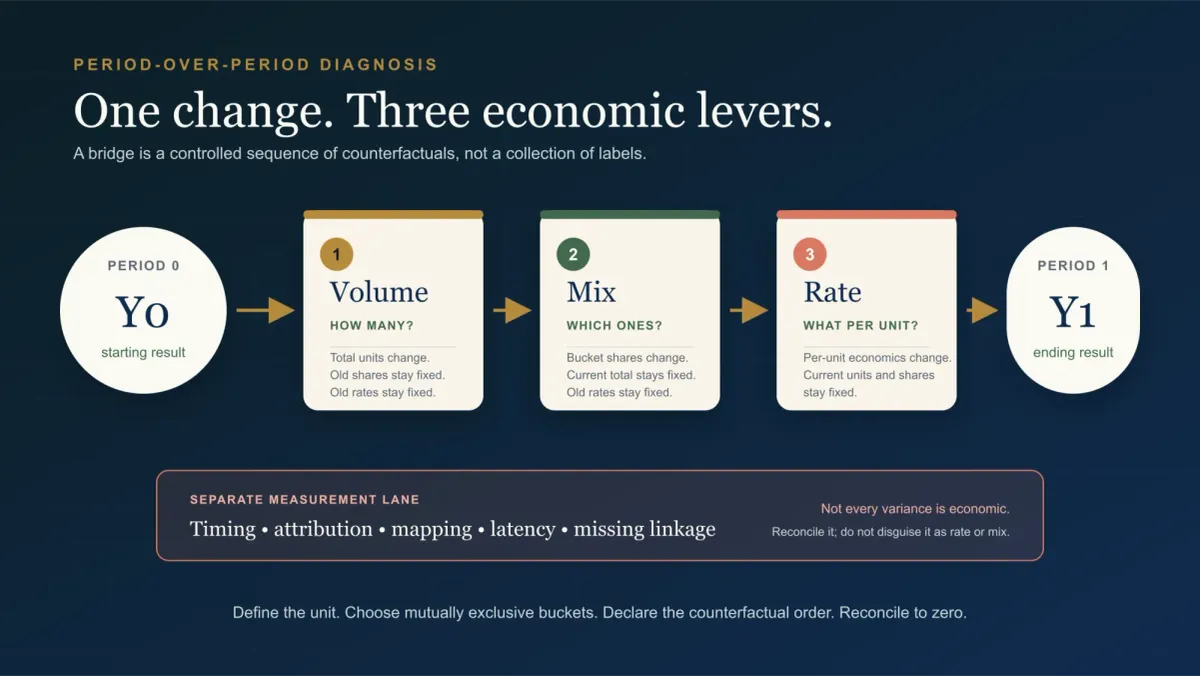
The objective: After reading this, you should be able to take the same metric measured in two periods, decide whether it can be decomposed validly, define the right unit and buckets, and quantify its movement as volume, mix, rate, or a separately identified reporting, scope, or measurement effect. You should also know when the decomposition is impossible, misleading, or dependent on a policy choice.

One number moved. That does not mean one thing happened.

Revenue can rise because the business served more units, because it served a more valuable combination of units, or because it earned more from comparable units. Cost can fall while every operating rate gets worse. Margin can decline while every product's margin improves. A data pipeline can create a variance even when the underlying economics did not move at all.

Rate-volume-mix analysis is how we stop saying the metric changed and start quantifying what changed underneath it.

It is not a magic finance template. It is a disciplined sequence of counterfactual questions:

1. What if only the total number of units had changed?
2. What if the composition of those units had then changed?
3. What if the economics inside each comparable bucket had then changed?
4. What reporting, scope, or measurement effects remain between the reconstructed and reported answers?

That sequence is the heart of the method.

The entire mental model in four questions

Before opening a spreadsheet, force four definitions.

Lens	The question	What changes	What stays fixed
Volume	How many?	Total units	Bucket shares and within-bucket rates
Mix	Which ones?	The share of units in each bucket	Total units and within-bucket rates
Rate	What per unit?	Economics inside comparable buckets	Current units and current bucket shares
Reconciliation	Did the report measure the same scope and reality?	Timing, translation, scope, mapping, attribution, or lineage	The normalized operating bridge

The shortest useful version is:

Volume is a bigger or smaller business. Mix is a different basket. Rate is different economics inside the same basket.

If heavier packages become a larger share of shipments, that is usually mix. If the same weight class costs more to handle, that is rate. If last month's shipment is recognized this month, that is timing. If a shipment cannot be linked to its cost, that is attribution.

These are diagnostic lenses, not independent laws of nature. Their usefulness depends on the unit, bucket structure, and counterfactual convention you choose.

The one identity that makes the bridge possible

For an additive outcome representable at the chosen grain as quantity times rate, write the period's result as:

where:

• q_i,t is the quantity in bucket i during period t;
• r_i,t is the outcome per unit in that bucket; and
• Y_t is the total outcome: revenue, cost, gross profit, emissions, labor hours, support spend, or another additive result.

Now separate bucket quantity into total volume and bucket share:

So:

This expression contains the three levers:

• Q is volume;
• w is mix; and
• r is rate.

That is most of the subject. The rest is choosing sound definitions, handling interactions honestly, and refusing to force separate reconciliation effects into operating labels.

Build four states, not three labels

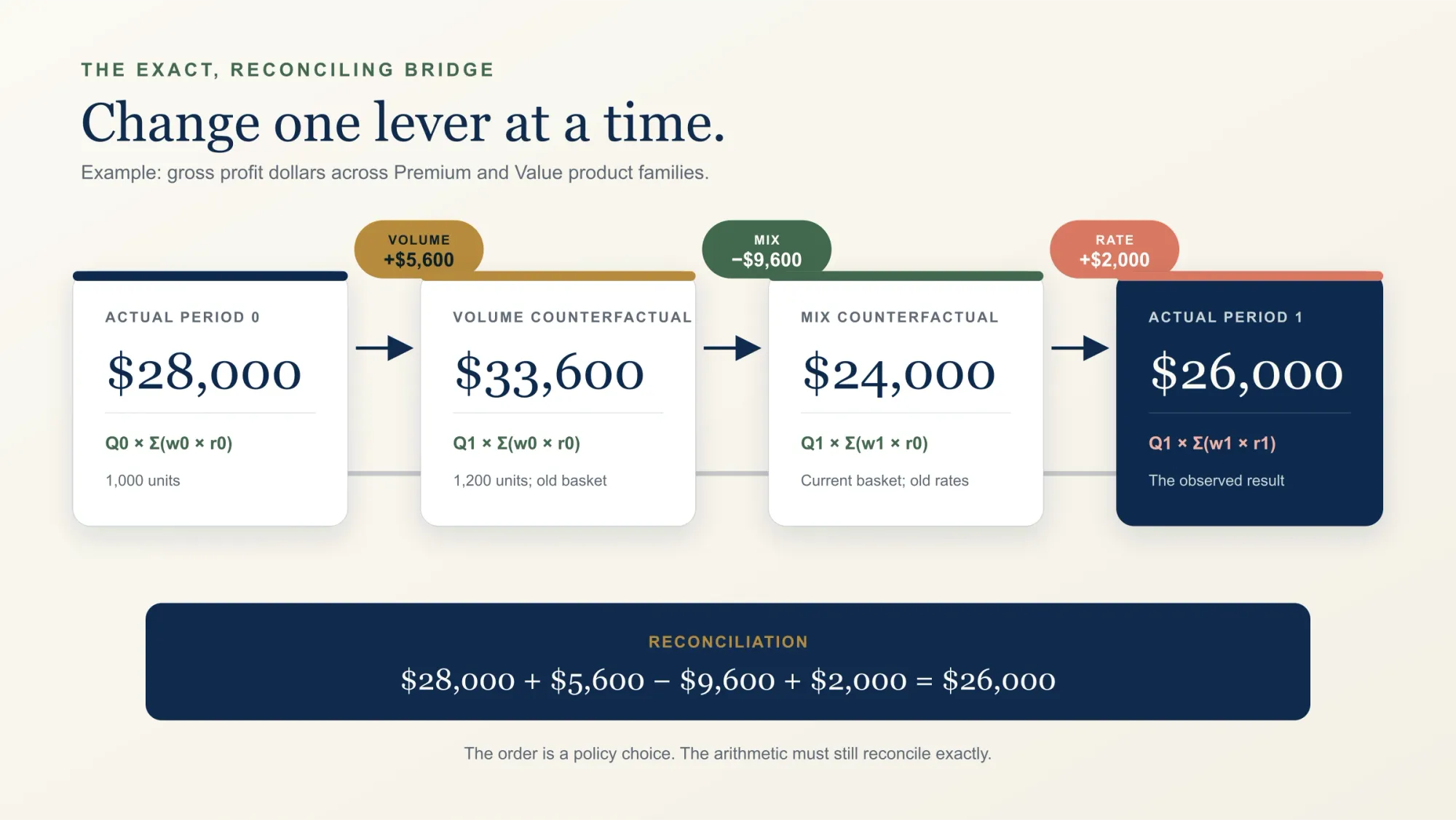
Suppose period 0 is the baseline and period 1 is the comparison. Use a declared volume → mix → rate sequence:

State	Volume	Mix	Rate	Meaning
Period 0 actual	Q₀	w₀	r₀	The observed starting result
Volume counterfactual	Q₁	w₀	r₀	Current total units, old basket, old economics
Mix counterfactual	Q₁	w₁	r₀	Current total units and basket, old economics
Period 1 actual	Q₁	w₁	r₁	The observed ending result

Each step changes exactly one lever:

Because the changes in bucket shares sum to zero, the same mix term can be centered on the old blended rate:

That version makes the sign intuitive: mix increases the chosen metric when share moves toward buckets whose baseline rate is above the baseline average. Whether that is favorable depends on the metric's declared sign convention.

Therefore:

This bridge reconciles exactly because it walks from one fully specified state to the next.

A crucial disclosure: the order is a convention

Changing volume, mix, and rate simultaneously creates interaction effects. If you change rate before mix, some dollars assigned to rate in the sequence above will move to mix. Both bridges can reconcile and still report different attribution.

That is not a flaw to conceal. It is a policy choice to disclose.

• Use a consistent ordered bridge when the organization wants an operational story it can reproduce every month.
• Use an order-neutral method, such as averaging each lever's marginal contribution across all six possible sequences, when credit, blame, or incentive compensation makes the ordering consequential. That is a Shapley-style decomposition.
• Never describe an order-dependent bridge as the uniquely true causal answer.

The World Bank's explanation of Shapley decomposition in Annex 4A, p. 54 uses the same core idea: change one factor in a counterfactual, calculate its marginal contribution, and average over possible sequences when order neutrality matters.

Worked example: gross profit per unit rose in every product family, yet total gross profit fell

Consider two product families. Gross profit per unit is selling price minus product cost.

Product	P0 units	P0 price	P0 cost	P0 profit/unit	P1 units	P1 price	P1 cost	P1 profit/unit
Premium	600	$100	$60	$40	400	$105	$62	$43
Value	400	$50	$40	$10	800	$52	$41	$11
Total	1,000			$28,000 profit	1,200			$26,000 profit

Three statements are simultaneously true:

• Total units increased by 20%.
• Unit profit improved in both families.
• Total gross profit fell by $2,000.

The bridge explains the apparent contradiction.

1. Volume: +$5,600

Period 0 earned an average of $28 gross profit per unit. Two hundred additional units at the old mix and old economics would add:

2. Mix: -$9,600

Premium fell from 60% of units to one-third; Value rose from 40% to two-thirds. Reweighting 1,200 units to that current mix, while retaining old bucket rates, removes $9,600.

This is not a claim that Value is a bad product. It is a claim that, at these unit economics, shifting toward Value reduced total gross profit relative to holding the old basket constant.

3. Rate: +$2,000

At current quantities, the two bucket contributions are:

Total rate effect: +$2,000.

4. Reconcile

The managerial story is precise: growth and better unit economics helped, but the shift toward the lower-profit product family more than offset both.

Rate can itself be a composite metric

“Rate” does not have to mean list price. It means the within-bucket change in the per-unit outcome.

In the example:

The +$2,000 rate step can therefore be decomposed again. Price and product cost are additive components of unit gross profit, so this second-level split introduces no interaction-allocation issue:

Within-bucket component	Calculation at current units	Effect on gross profit
Selling price	400 × $5 + 800 × $2	+$3,600
Product cost	−(400 × $2 + 800 × $1)	-$1,600
Net rate effect		+$2,000

For contribution profit, the rate tree might go deeper:

Each component remains signed according to its effect on the chosen result. A higher selling price helps profit; a higher product cost hurts it. Define that sign convention before calculating the bridge.

This recursive idea is powerful. The top bridge answers volume, mix, or within-bucket economics? The next bridge answers which component of within-bucket economics? A further operational drill-down may separate wage, productivity, rework, and process-path effects.

Do not bury fixed costs inside a fictional per-unit rate without stating the assumption. Fixed cost, capacity utilization, and absorption often deserve their own bridge or a separate line below contribution profit.

Why percentages require different discipline

Gross profit dollars are additive. Gross margin percentage is a ratio:

A pure weighted average can be written as:

There is no standalone volume effect on a pure average. If every bucket doubles with identical proportions, the average does not change. For a percentage, bridge the numerator and denominator separately to understand their dollar or count movements. If you allocate the percentage-point change, recompute the ratio at each declared counterfactual state; do not divide each dollar effect by one convenient denominator.

For a ratio of sums, the correct bucket weight is the bucket's share of the denominator. Gross-margin percentages are revenue-weighted; conversion rates are eligible-visit-weighted; defect rates are inspected-unit-weighted. A simple average of bucket percentages is generally wrong.

Our example makes the danger vivid:

• Premium margin improves from 40.0% to about 41.0%.
• Value margin improves from 20.0% to about 21.2%.
• Total gross margin falls from 35.0% to about 31.1%.

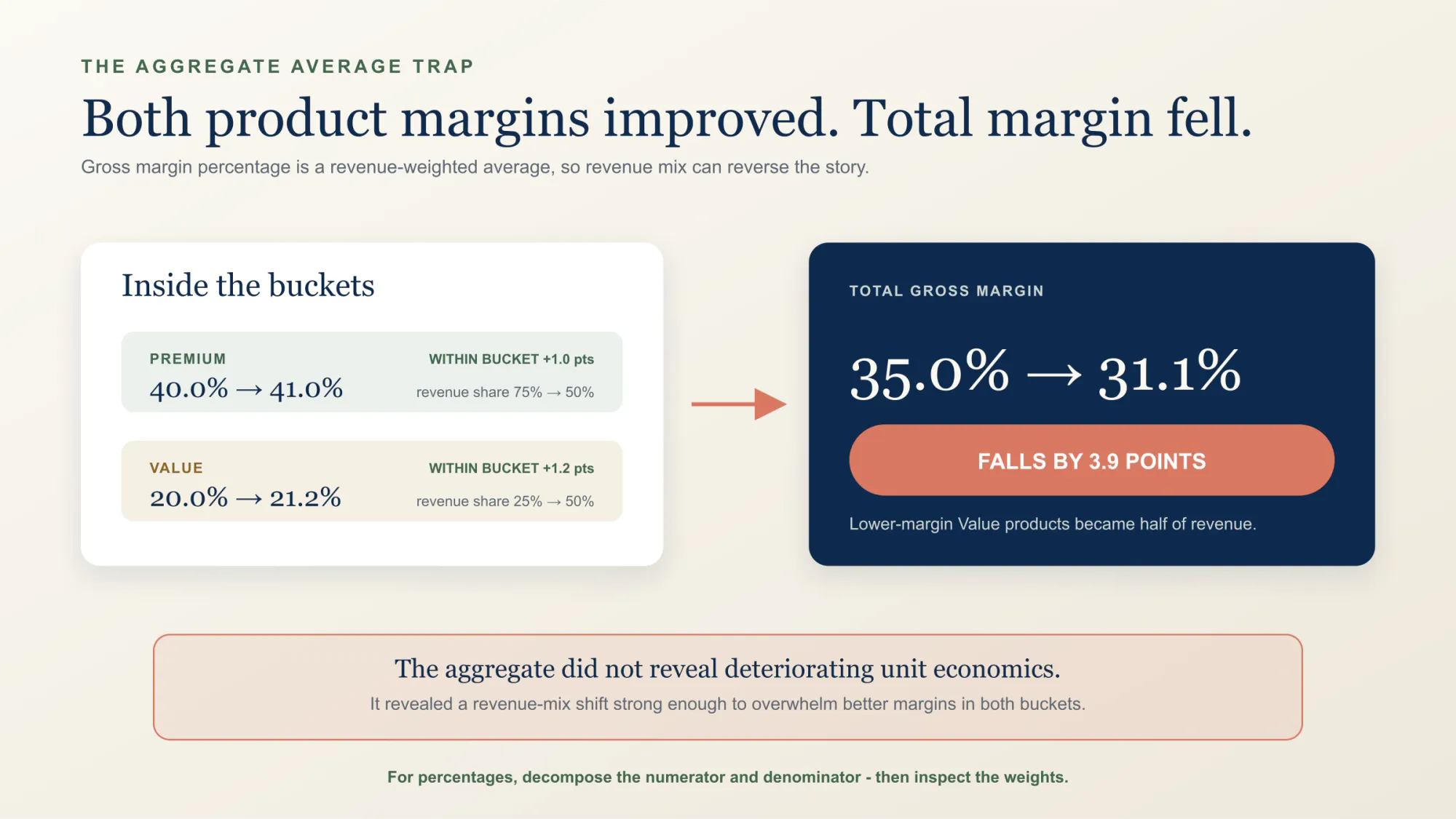
This is a Simpson-type aggregation reversal: the total moves opposite the subgroups because the weights changed. Simpson's original 1951 paper, “The Interpretation of Interaction in Contingency Tables”, is the classic reference for the broader aggregation phenomenon.

The lesson is not that averages are useless. It is that an aggregate average cannot tell you whether the movement occurred inside buckets or between buckets.

Medians, percentiles, retention, inventory turns, and other nonlinear statistics need an explicit counterfactual function. Do not force them into ∑ (quantity × rate). Recalculate the statistic on controlled counterfactual populations, or choose an additive numerator-and-denominator formulation that matches the decision.

The bucket dimension is part of the hypothesis

“Mix got worse” is incomplete until someone answers:

• Mix of what unit?
• Across which mutually exclusive buckets?
• Why should those buckets have structurally different economics?
• Which buckets gained and lost share?
• What were their rates in both periods?

For fulfillment cost, product category may be explanatory—or it may be decorative. The real driver could be package size, handling path, service speed, facility type, geography, automation level, or some interaction among them.

A useful bucket structure is:

• mutually exclusive: one unit does not land in two buckets;
• collectively exhaustive: every in-scope unit lands somewhere;
• stable across periods: classification did not silently change;
• economically meaningful: rates differ for a reason you can act on; and
• available at the same grain and clock as the metric.

Do not calculate mix independently by product, region, channel, and customer type and then add the four answers. Those dimensions overlap; summing them double-counts the same movement. Use a governed hierarchy, a single joint bucket definition, or a multivariate attribution method.

Official price-and-volume measurement guidance makes the same point in a different setting: grouping choices must match the measurement purpose, and the unit must represent output rather than an unrelated input. See the OECD/Eurostat/WHO health-account chapter on price and volume measures and the IMF's Consumer Price Index Manual: Theory, 2025.

Keep reporting, scope, and measurement effects outside the operating bridge

Sometimes the reported metric does not equal the result reconstructed from consistently defined units and rates. Define Normalized_t as the period's result recomputed under a common grain, bucket mapping, scope, currency convention, and recognition policy. The rate-volume-mix bridge explains the change in that normalized operating result.

Then reconcile the normalized bridge to the reported change explicitly:

Translation and scope effects are real reported movements, not necessarily errors. Examples include currency translation, acquisitions, disposals, geographic-perimeter changes, or a deliberate change in denominator coverage. Keep them separate because they answer a different question from operating rate, volume, and mix.

After identifying those effects, define the remaining measurement and timing residual for each period as:

That residual can include activity-date versus accounting-date timing, accrual versus application timing, missing or delayed linkage, unremapped taxonomy changes, late-arriving data, or manual adjustments.

Name every separate effect and quantify it. Assign an owner and expected unwind date when the difference should unwind. Do not make rate or mix absorb whatever the operating model could not explain.

New and discontinued products are different: they are real economic entry and exit effects, but they lack a naturally observed rate in one period. Show them as a separate entry/exit line, or disclose the comparable benchmark used to place them in rate or mix.

An unexplained residual is not analytical sophistication. It is a reconciliation problem.

Ten ways a plausible bridge becomes wrong

1. Calling volume “mix.” More units is volume. A different share of unit types is mix. Both can move at once.
2. Calling a blended average “rate.” First inspect within-bucket rates. The average may have moved only because the weights changed.
3. Using the wrong denominator. Labor cost per shipment item answers a different question from labor cost per inventory unit handled.
4. Averaging averages. Within a bucket, divide the sum of outcomes by the sum of units unless every lower-level observation truly deserves equal weight.
5. Changing bucket definitions between periods. Reclassification can masquerade as mix.
6. Hiding interaction allocation. Declare the bridge order or use an order-neutral method.
7. Forcing ratios into an additive bridge. Decompose numerator and denominator, then recompute the ratio at each declared counterfactual state.
8. Mistaking the bridge for causality. A bridge localizes the movement. It does not prove why price, productivity, mix, or demand changed.
9. Treating entry and exit as an ordinary comparison. New or discontinued buckets need a declared benchmark or a separate effect.
10. Forcing nonlinear statistics into quantity × rate. Recompute the metric on controlled populations instead.

The operating sequence: eight questions

Everything above condenses into one field checklist. These eight questions connect the definitions, counterfactuals, caveats, and reconciliation—and capture most of what a working analyst needs when the same metric appears in two periods.

1. Decision and metric: What decision will this inform, what does the sign mean, and is the outcome additive, a ratio, or nonlinear?
2. Unit and scope: What exactly are we counting, on which clock, in which currency, and across which entities?
3. Buckets: Are the categories mutually exclusive, collectively exhaustive, stable, economically different, and actionable?
4. Volume: How much of the movement comes from a change in total activity while old mix and rates stay fixed?
5. Mix: How much comes from changed bucket shares while current total activity and old rates stay fixed?
6. Rate: How much comes from changed outcomes per unit inside comparable buckets?
7. Convention and reconciliation: What order allocates interactions, do ratios get recomputed at each state, and does the normalized bridge plus reporting, scope, and measurement effects land exactly on the reported result?
8. Action and communication: Which material driver is controllable, where should it be decomposed again, and what one sentence states the result, convention, and decision?

If a bridge cannot survive those eight questions, it is not ready for a decision meeting.

Practice lab: five unfamiliar applications

Now apply that sequence to five domains where the unit and bucket choices are less obvious. For every row below:

1. calculate Y₀ and Y₁;
2. calculate volume, mix, and rate using the volume → mix → rate order;
3. name one plausible reporting, scope, or measurement effect; and
4. write one action that follows from the largest economic driver.

Positive and negative mean “increased” and “decreased” the stated metric—not automatically “good” and “bad.”

Scenario and metric	Total volume Q₀ → Q₁	Bucket A: w₀ → w₁; r₀ → r₁	Bucket B: w₀ → w₁; r₀ → r₁
Cloud compute spend	10,000 → 12,000 normalized compute-hours	On-demand: 60% → 40%; $0.12 → $0.13/hour	Reserved: 40% → 60%; $0.07 → $0.065/hour
Hospital labor cost	1,000 → 1,100 encounters	Routine: 70% → 60%; $80 → $76/encounter	Complex: 30% → 40%; $240 → $228/encounter
Electricity emissions	100 → 120 MWh	Fossil-intensive supply: 40% → 25%; 0.80 → 0.70 tCO2e/MWh	Low-carbon supply: 60% → 75%; 0.20 → 0.15 tCO2e/MWh
Customer-support cost	10,000 → 9,000 resolved cases	Simple: 80% → 65%; $4.00 → $3.50/case	Complex: 20% → 35%; $20 → $18/case
Portfolio annualized interest income	$1.0m → $1.2m invested balance	Cash: 40% → 20%; 4.0% → 3.5% annualized yield	Bonds: 60% → 80%; 5.0% → 5.5% annualized yield

Work the five bridges before reading on; the value lies in choosing the right unit, buckets, and interpretation—not merely checking the arithmetic.

Answer key

Scenario	Y₀ → Y₁	Volume	Mix	Rate	Net change (V + M + R)	Residual
Cloud compute spend	$1,000 → $1,092	+$200	-$120	+$12	+$92	0
Hospital labor cost	$128,000 → $150,480	+$12,800	+$17,600	-$7,920	+$22,480	0
Electricity emissions	44.0 → 34.5 tCO2e	+8.8	-10.8	-7.5	-9.5	0
Customer-support cost	$72,000 → $77,175	-$7,200	+$21,600	-$9,225	+$5,175	0
Portfolio annualized interest income	$46,000 → $61,200	+$9,200	+$2,400	+$3,600	+$15,200	0

Possible reconciliation effects include delayed cloud-credit amortization, a hospital coding backlog, renewable-certificate accounting, a changed “resolved case” definition, or accrued-interest and currency timing. None is present in the clean practice data; your job is to know where each could enter a real bridge and whether it is an operating, scope, or measurement effect.

Notice the stories:

• Cloud volume raises spend, purchasing mix offsets much of it, and within-model rates add little.
• Hospital rates improve, but higher volume and more complex encounters dominate.
• Electricity demand rises, yet cleaner supply mix and lower emission factors reduce total emissions.
• Support handles fewer cases and becomes cheaper within each class, but a surge in complex cases still raises total cost.
• Portfolio scale, asset allocation, and yields all contribute positively to interest income.

The same method travels because it is not really about finance. It is about how much activity occurred, which buckets it fell into, and the outcome per unit inside each bucket.

The final discipline is linguistic. Never say merely, “mix was unfavorable” or “rate improved.” Say which unit, which bucket, which per-unit component, how much it contributed, which convention assigned it, and what decision follows.

Then the bridge stops being a chart.

It becomes an explanation.